How the velocity estimator works
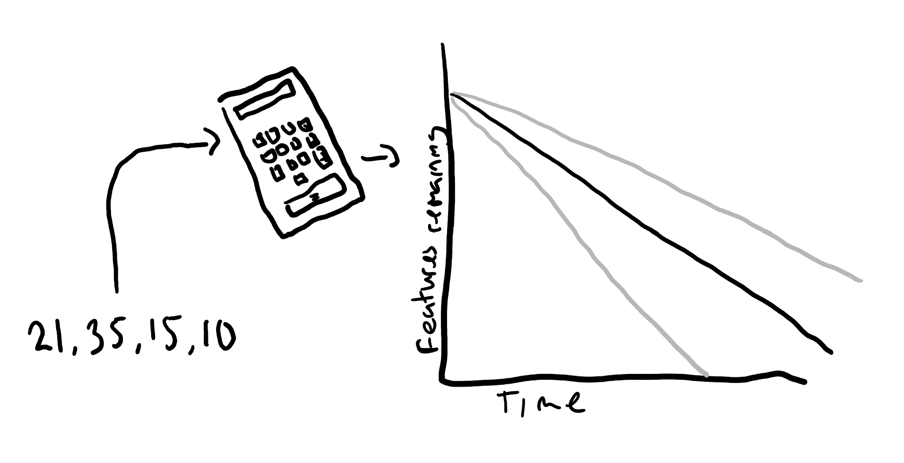
Many software teams track their velocity, use this handy calculator to discover your chances of delivering a certain amount of story points.
Let’s talk about how the velocity calculator works behind the scenes.
The Idea
I saw a forecast diagram with a growing cone, for the number of features to be delivered over the course of the project (like the one above) and started to wonder how that was calculated. Was the lower and upper bounds plucked out of thin air or did they use a model? I had a search and couldn’t find anything so devised one myself.
Major Concepts
We feed your previous velocities into the Student’s t-distribution. I settled on using this distribution after a fair amount of research and trial and error of which distribution to use. Mainly because this allows the use of small sample sizes compared to something like the normal distribution.
It calculates the mean, the confidence interval and the distribution curve (displayed in the table).
The confidence interval is really a best guess at the segment that contains the population mean based on how confident you wish to be.
The distribution curve shows, for a given number of points, the estimated chance of delivering them. It’s probably my favorite aspect as I like viewing the chances of delivering certain amounts of points. It would be interesting in a planning session to say there’s a 10% risk if we bring in those points.
Back to the distribution, it’s not perfect as we will see below.
Assumptions
This model has some baked in assumptions:
- The underlying distribution is normal curve.
- That the scale of measurement is continuous.
- It’s a random sample.
- The population mean doesn’t change.
For the first point, I have assumed that teams deliver in a normally distributed fashion. It would be interesting to graph some long-running data (I might do that in a future blog post if I can get my hands on good data).
I’m not sure if the scale is continuous or not. As the Fibonacci scale is often used to point items, which isn’t continuous, this presents an issue. However, it’s “more continuous” (I might be showing the limits of my stats knowledge here) than rugby scores, since you could complete multiple stories with a value of one, whereas in rugby some numbers such as 1 are impossible to score.
I’m not sure if the last couple of sprints is the best random sample, as they are likely to be influenced by similar factors. On the other hand, as point four touches on, we normally assume population mean (base velocity) doesn’t change. Whereas we know the velocity does change over time; if the velocity is actually changing (hopefully getting better) then a sprints velocity from a long time ago is not good data either.
Overall Thoughts
I think the calculator probably has some problems with its statistical model, but for the accuracy required from it, I’m willing to set these problems aside.